5.5 Application Problems with Exponential and Logarithmic Functions
Strategies for Solving Equations That Contain Exponents
When you're working with real-world problems involving exponential and logarithmic functions, the key to solving them is figuring out where the variable is located in the equation. Is it in the exponent? Is it the base? Is it a coefficient? Each position requires a different solving strategy. Let's explore the four main strategies for tackling equations that contain exponents.
Why does variable position matter so much? Think about compound interest: if you're solving for the initial investment (coefficient), you use simple algebra. But if you're solving for time (exponent), you need logarithms. The math tool you need depends entirely on what you're trying to find.
The General Form
Suppose we have an equation in the form:
\[\text{value} = \text{coefficient} \times (\text{base})^{\text{exponent}}\]We consider four strategies for solving this equation, depending on which parts are known and which contain the variable.
The Four Strategies
STRATEGY A: If the coefficient, base, and exponent are all known, we only need to evaluate the expression \(\text{coefficient} \times (\text{base})^{\text{exponent}}\) to find its value.
STRATEGY B: If the variable is the coefficient, evaluate the expression for \((\text{base})^{\text{exponent}}\) first. Then it becomes a linear equation which we solve by dividing to isolate the variable.
STRATEGY C: If the variable is in the exponent, use logarithms to solve the equation.
STRATEGY D: If the variable is in the base (but not in the exponent), use roots to solve the equation.
Think of these strategies as a decision tree. First question: "Where's my variable?" Second question: "Which tool gets it out?" This systematic approach prevents you from getting stuck wondering how to start.
Below we examine each strategy with examples of its use.
Strategy A: Evaluating When All Values Are Known
If the coefficient, base, and exponent are all known, we only need to evaluate the expression \(\text{coefficient} \times (\text{base})^{\text{exponent}}\) to find its value.
Suppose that a stock's price is rising at the rate of \(7\%\) per year, and that it continues to increase at this rate. If the value of one share of this stock is $43 now, find the value of one share of this stock three years from now.
Example 5.5.1 Solution
Let \(y\) = the value of the stock after \(t\) years. We use the exponential growth model:
\[y = ab^t\]The problem tells us that \(a = 43\) (the initial value) and \(r = 0.07\) (the growth rate as a decimal), so:
\[b = 1 + r = 1 + 0.07 = 1.07\]Therefore, our function is:
\[y = 43(1.07)^t\]In this case we know that \(t = 3\) years, and we need to evaluate \(y\) when \(t = 3\).
At the end of 3 years, the value of this one share of stock will be:
\[y = 43(1.07)^3 = \$52.68\]This is Strategy A in action: we know everything (coefficient = 43, base = 1.07, exponent = 3), so we just calculate. This is the most straightforward scenario—you're simply plugging in numbers and computing the result.
Strategy B: Solving When the Variable Is the Coefficient
If the variable is the coefficient, evaluate the expression for \((\text{base})^{\text{exponent}}\) first. Then it becomes a linear equation which we solve by dividing to isolate the variable.
The value of a new car depreciates (decreases) after it is purchased. Suppose that the value of the car depreciates according to an exponential decay model. Suppose that the value of the car is $12,000 at the end of 5 years and that its value has been decreasing at the rate of \(9\%\) per year. Find the value of the car when it was new.
Example 5.5.2 Solution
Let \(y\) be the value of the car after \(t\) years. We use the exponential decay model:
\[y = ab^t\]Since the car is depreciating at \(9\%\) per year, we have:
\[r = -0.09 \quad \text{and} \quad b = 1 + r = 1 + (-0.09) = 0.91\]The function is:
\[y = a(0.91)^t\]In this case we know that when \(t = 5\), then \(y = 12000\). Substituting these values gives:
\[12000 = a(0.91)^5\]We need to solve for the initial value \(a\), which is the purchase price of the car when new.
Step 1: First evaluate \((0.91)^5\):
\[(0.91)^5 \approx 0.624\]Step 2: Now solve the resulting linear equation to find \(a\):
\[12000 = a(0.624)\] \[a = \frac{12000}{0.624} = \$19,230.77\]The car's value was $19,230.77 when it was new.
Notice how we transformed an exponential equation into a simple linear equation by evaluating the exponential part first. Once we calculated \((0.91)^5\), we were left with \(12000 = a \times 0.624\), which is just basic algebra. This is the power of Strategy B: reduce the problem to something simpler.
Why is this useful? Car dealerships, insurance companies, and tax assessors all need to work backwards from current value to original value. Strategy B is the tool they use. It's also how you'd calculate the original investment if you know how much your savings account is worth after several years of interest.
Strategy C: If the variable is in the exponent, use logarithms to solve the equation.
When the unknown variable appears in the exponent (like \(2^x = 16\)), we can't simply isolate it using basic algebra. This is where logarithms become essential—they're the mathematical tool that "brings down" exponents so we can solve for the variable. In real-world applications, this strategy helps us answer questions like "How long until my investment doubles?" or "When will a population reach a certain size?"
A national park has a population of 5000 deer in the year 2016. Conservationists are concerned because the deer population is decreasing at the rate of \(7\%\) per year.
If the population continues to decrease at this rate, how long will it take until the population is only 3000 deer?
Example 5.5.3 Solution
Let's set up our exponential decay model. Let \(y\) be the number of deer in the national park \(t\) years after the year 2016. We use the exponential model:
\[y = ab^{t}\]First, we identify our values:
- The decay rate is \(r = -0.07\) (negative because the population is decreasing)
- The base is \(b = 1 + r = 1 + (-0.07) = 0.93\)
- The initial population is \(a = 5000\)
This gives us the exponential decay function:
\[y = 5000(0.93)^{t}\]To find when the population will be 3000, we substitute \(y = 3000\):
\[3000 = 5000(0.93)^{t}\]Next, divide both sides by 5000 to isolate the exponential expression:
\[\frac{3000}{5000} = \frac{5000}{5000}(0.93)^{t}\] \[0.6 = 0.93^{t}\]Notice how we isolated the exponential term before applying logarithms. This is a crucial step—we want the exponential expression by itself on one side of the equation before we "unlock" the exponent using logarithms.
Now we rewrite the equation in logarithmic form, then use the change of base formula to evaluate:
\[t = \log_{0.93}(0.6)\]Using the change of base formula with natural logarithms:
\[t = \frac{\ln(0.6)}{\ln(0.93)} = 7.039 \text{ years}\]Answer: After approximately 7.039 years, the deer population will decline to 3000.
Important Note about Precision: In this example, we needed to state the answer to several decimal places to remain accurate. Let's see why:
If we round to \(t = 7\) years and evaluate the original function:
\[y = 5000(0.93)^{7} = 3008.5 \text{ deer}\]This is close to 3000, but not exactly 3000. However, using \(t = 7.039\) years produces:
\[y = 5000(0.93)^{7.039} = 3000.0016 \approx 3000 \text{ deer}\]Why does precision matter here? In real-world conservation planning, accurate timing is critical. If park managers need to implement intervention strategies when the population hits 3000, being off by even a few days could mean the difference between a successful intervention and missing the optimal window. This is why we keep extra decimal places in our calculations—rounding too early can compound errors.
A video posted on YouTube initially had 80 views as soon as it was posted. The total number of views to date has been increasing exponentially according to the exponential growth function \(y = 80e^{0.12t}\), where \(t\) represents time measured in days since the video was posted.
How many days does it take until 2500 people have viewed this video?
Example 5.5.4 Solution
Let \(y\) be the total number of views \(t\) days after the video is initially posted.
We are given that the exponential growth function is \(y = 80e^{0.12t}\) and we want to find the value of \(t\) for which \(y = 2500\).
Substitute \(y = 2500\) into the equation:
\[2500 = 80e^{0.12t}\]Divide both sides by the coefficient, 80, to isolate the exponential expression:
\[\frac{2500}{80} = \frac{80}{80}e^{0.12t}\] \[31.25 = e^{0.12t}\]When we have the natural base \(e\) in our exponential equation, we use the natural logarithm (ln) to solve it. This is because ln and \(e\) are inverse operations—they "undo" each other, just like multiplication and division.
Rewrite the equation in logarithmic form:
\[0.12t = \ln(31.25)\]Divide both sides by 0.12 to isolate \(t\), then use your calculator's natural log function to evaluate:
\[t = \frac{\ln(31.25)}{0.12}\] \[t = \frac{3.442}{0.12}\] \[t \approx 28.7 \text{ days}\]Answer: This video will have 2500 total views approximately 28.7 days after it was posted.
Exponential growth models like this are everywhere in the digital age. Content creators, marketers, and social media analysts use these models to predict when a video will go viral, when to boost advertising, or when engagement will plateau. Understanding how to solve these equations gives you the power to make data-driven decisions about timing and strategy in the digital marketplace.
Strategy D: If the variable is not in the exponent, but is in the base, we use roots to solve the equation.
This is a crucial distinction: logarithms are only for when the variable is in the exponent (like \(2^x = 8\)). When the variable is in the base (like \(x^2 = 8\)), we use roots instead. Think of it this way: if you're asking "what number raised to a power gives me this result?", use roots. If you're asking "what power do I raise this number to?", use logarithms.
It is important to remember that we only use logarithms when the variable is in the exponent.
A statistician creates a website to analyze sports statistics. His business plan states that his goal is to accumulate 50,000 followers by the end of 2 years (24 months from now). He hopes that if he achieves this goal his site will be purchased by a sports news outlet. The initial user base of people signed up as a result of pre-launch advertising is 400 people.
Find the monthly growth rate needed if the user base is to accumulate to 50,000 users at the end of 24 months.
Example 5.5.5 Solution
Let \(y\) be the total user base \(t\) months after the site is launched.
The growth function for this site is \(y = 400(1 + r)^{t}\)
We don't know the growth rate \(r\). We do know that when \(t = 24\) months, then \(y = 50000\). Substitute the values of \(y\) and \(t\); then we need to solve for \(r\).
\[50000 = 400(1 + r)^{24}\]Divide both sides by 400 to isolate \((1+r)^{24}\) on one side of the equation:
\[\frac{50000}{400} = \frac{400}{400}(1 + r)^{24}\] \[125 = (1 + r)^{24}\]Because the variable in this equation is in the base, we use roots:
\[\sqrt[24]{125} = 1 + r\] \[125^{1/24} = 1 + r\] \[1.2228 \approx 1 + r\] \[0.2228 \approx r\]The website's user base needs to increase at the rate of \(22.28\%\) per month in order to accumulate 50,000 users by the end of 24 months.
This growth rate of 22.28% per month is extremely aggressive! For context, most successful social media platforms grow at 5-15% per month in their early stages. This example shows why realistic business planning is crucial—the statistician might need to revise his timeline or find additional marketing strategies to achieve this goal.
A fact sheet on caffeine dependence from Johns Hopkins Medical Center states that the half life of caffeine in the body is between 4 and 6 hours. Assuming that the typical half life of caffeine in the body is 5 hours for the average person and that a typical cup of coffee has \(120\mathrm{mg}\) of caffeine.
- Write the decay function.
- Find the hourly rate at which caffeine leaves the body.
- How long does it take until only \(20\mathrm{mg}\) of caffeine is still in the body?
Hopkins Medicine Caffeine Dependence Fact Sheet
Example 5.5.6 Solution
Part a. Let \(y\) be the total amount of caffeine in the body \(t\) hours after drinking the coffee.
The exponential decay function \(y = ab^{t}\) models this situation.
The initial amount of caffeine is \(a = 120\).
We don't know \(b\) or \(r\), but we know that the half-life of caffeine in the body is 5 hours. This tells us that when \(t = 5\), then there is half the initial amount of caffeine remaining in the body.
\[\begin{array}{l} y = 120b^{t} \\ \frac{1}{2}(120) = 120b^{5} \\ 60 = 120b^{5} \end{array}\]Divide both sides by 120 to isolate the expression \(b^5\) that contains the variable:
\[\begin{array}{l} \frac{60}{120} = \frac{120}{120}b^{5} \\ 0.5 = b^{5} \end{array}\]The variable is in the base and the exponent is a number. Use roots to solve for \(b\):
\[\begin{array}{l} \sqrt[5]{0.5} = b \\ 0.5^{1/5} = b \\ 0.87 = b \end{array}\]We can now write the decay function for the amount of caffeine (in mg) remaining in the body \(t\) hours after drinking a cup of coffee with \(120\mathrm{mg}\) of caffeine:
\[y = f(t) = 120(0.87)^{t}\]Part b. Use \(b = 1 + r\) to find the decay rate \(r\). Because \(b = 0.87 < 1\) and the amount of caffeine in the body is decreasing over time, the value of \(r\) will be negative.
\[\begin{array}{l} 0.87 = 1 + r \\ r = -0.13 \end{array}\]The decay rate is \(13\%\); the amount of caffeine in the body decreases by \(13\%\) per hour.
This explains why you might feel jittery for hours after drinking coffee! Even though caffeine decays at 13% per hour, it takes a long time to fully leave your system. This is why doctors recommend avoiding caffeine 6-8 hours before bedtime.
Part c. To find the time at which only \(20\mathrm{mg}\) of caffeine remains in the body, substitute \(y = 20\) and solve for the corresponding value of \(t\).
\[\begin{array}{l} y = 120(.87)^{t} \\ 20 = 120(.87)^{t} \end{array}\]Divide both sides by 120 to isolate the exponential expression:
\[\begin{array}{l} \frac{20}{120} = \frac{120}{120}\left(.87^{t}\right) \\ 0.1667 = .87^{t} \end{array}\]Rewrite the expression in logarithmic form and use the change of base formula:
\[\begin{array}{l} t = \log_{0.87}(0.1667) \\ t = \frac{\ln(0.1667)}{\ln(0.87)} \approx 12.9 \text{ hours} \end{array}\]After 12.9 hours, \(20\mathrm{mg}\) of caffeine remains in the body.
Notice how we switched strategies in part c! We started with the variable in the base (parts a and b), but in part c, the variable moved to the exponent. Once we had the decay function \(y = 120(0.87)^t\), solving for \(t\) required logarithms because now \(t\) is in the exponent. This shows why understanding when to use roots versus logarithms is so important.
Expressing Exponential Functions in the Forms \(y = ab^{t}\) and \(y = ae^{kt}\)
Now that we've developed our equation solving skills, we revisit the question of expressing exponential functions equivalently in the forms \(y = ab^{t}\) and \(y = ae^{kt}\).
Why do we need two different forms for the same function? The form \(y = ab^t\) is intuitive—it directly shows the growth factor \(b\) per time period. The form \(y = ae^{kt}\) is preferred in calculus and advanced applications because the number \(e\) (approximately 2.718) has special mathematical properties that make derivatives and integrals simpler. Being able to convert between these forms is essential for different contexts.
We've already determined that if given the form \(y = ae^{kt}\), it is straightforward to find \(b\).
For the following examples, assume \(t\) is measured in years.
- Express \(y = 3500e^{0.25t}\) in form \(y = ab^t\) and find the annual percentage growth rate.
- Express \(y = 28000e^{-0.32t}\) in form \(y = ab^t\) and find the annual percentage decay rate.
Example 5.5.7 Solution
Part a. Express \(y = 3500e^{0.25t}\) in the form \(y = ab^t\).
\[y = ae^{kt} = ab^{t}\] \[a(e^{k})^{t} = ab^{t}\]Thus \(e^{k} = b\)
In this example, \(b = e^{0.25} \approx 1.284\)
We rewrite the growth function as \(y = 3500(1.284^{t})\)
To find \(r\), recall that \(b = 1 + r\):
\[\begin{array}{l} 1.284 = 1 + r \\ 0.284 = r \end{array}\]The continuous growth rate is \(k = 0.25\) and the annual percentage growth rate is \(28.4\%\) per year.
Part b. Express \(y = 28000e^{-0.32t}\) in the form \(y = ab^t\)
\[y = ae^{kt} = ab^{t}\] \[a(e^{k})^{t} = ab^{t}\]Thus \(e^{k} = b\)
In this example, \(b = e^{-0.32} \approx 0.7261\)
We rewrite the growth function as \(y = 28000(0.7261^{t})\)
To find \(r\), recall that \(b = 1 + r\):
\[\begin{array}{l} 0.7261 = 1 + r \\ -0.2739 = r \end{array}\]The continuous decay rate is \(k = -0.32\) and the annual percentage decay rate is \(27.39\%\) per year.
Notice that in the sentence above, we omit the negative sign when stating the annual percentage decay rate because we have used the word "decay" to indicate that \(r\) is negative. This is a common convention—when we say something "decays at 27.39%", the negative is implied. However, in the equation, we must write \(r = -0.2739\) to maintain mathematical accuracy.
a. Express \(y = 4200(1.078)^{t}\) in the form \(y = ae^{kt}\).
b. Express \(y = 150(0.73)^{t}\) in the form \(y = ae^{kt}\).
Example 5.5.8 Solution
Part a. Express \(y = 4200(1.078)^{t}\) in the form \(y = ae^{kt}\).
\[y = ae^{kt} = ab^{t}\] \[a\left(e^{k}\right)^{t} = ab^{t}\] \[e^{k} = b\] \[e^{k} = 1.078\]Therefore \(k = \ln 1.078 \approx 0.0751\)
We rewrite the growth function as \(y = 4200e^{0.0751t}\)
Notice the key step: when we have \(e^k = b\), we take the natural logarithm of both sides to solve for \(k\). This gives us \(k = \ln(b)\). This is the reverse process of Example 2.7, where we had \(k\) and found \(b\) using \(b = e^k\).
Part b. Express \(y = 150(0.73)^{t}\) in the form \(y = ae^{kt}\)
\[y = ae^{kt} = ab^{t}\] \[a\left(e^{k}\right)^{t} = ab^{t}\] \[e^{k} = b\] \[e^{k} = 0.73\]Therefore \(k = \ln 0.73 \approx -0.3147\)
We rewrite the decay function as \(y = 150e^{-0.3147t}\)
Converting between these two forms is a fundamental skill in applied mathematics. In business and finance, you'll often see the \(y = ab^t\) form because it's easier to interpret (e.g., "the investment grows by a factor of 1.078 each year"). In physics, biology, and engineering, you'll see the \(y = ae^{kt}\) form because it simplifies calculus operations. Being fluent in both forms makes you versatile across different fields.
An Application of a Logarithmic Function
Suppose we invest $10,000 today and want to know how long it will take to accumulate to a specified amount, such as $15,000. The time \(t\) needed to reach a future value \(y\) is a logarithmic function of the future value: \(t = g(y)\).
Why does this matter? When you're planning for retirement, saving for a house, or building an emergency fund, you don't just want to know "how much will I have?" You also want to know "how long until I reach my goal?" This is where logarithmic functions become incredibly practical—they let you work backwards from your target amount to find out how many years you'll need to wait.
Suppose that Vinh invests $10,000 in an investment earning \(5\%\) per year. He wants to know how long it would take his investment to accumulate to $12,000, and how long it would take to accumulate to $15,000.
Example 5.5.9 Solution
We start by writing the exponential growth function that models the value of this investment as a function of the time since the $10,000 is initially invested:
\[y = 10000(1.05)^{t}\]We divide both sides by 10,000 to isolate the exponential expression on one side:
\[\frac{y}{10000} = 1.05^{t}\]Next we rewrite this in logarithmic form to express time as a function of the accumulated future value. We'll use function notation and call this function \(g(y)\):
\[t = g(y) = \log_{1.05}\left(\frac{y}{10000}\right)\]Notice what we just did—we "flipped" the exponential equation to solve for time instead of money. This is the power of logarithms: they let us answer the question "what exponent do I need?" instead of "what's the result of this exponent?"
We use the change of base formula to express \(t\) as a function of \(y\) using natural logarithm:
\[t = g(y) = \frac{\ln\left(\frac{y}{10000}\right)}{\ln(1.05)}\]We can now use this function to answer Vinh's questions.
To find the number of years until the value of this investment is $12,000, we substitute \(y = 12000\) into function \(g\) and evaluate \(t\):
\[t = g(12000) = \frac{\ln\left(\frac{12000}{10000}\right)}{\ln(1.05)} = \frac{\ln(1.2)}{\ln(1.05)} = 3.74 \text{ years}\]To find the number of years until the value of this investment is $15,000, we substitute \(y = 15000\) into function \(g\) and evaluate \(t\):
\[t = g(15000) = \frac{\ln\left(\frac{15000}{10000}\right)}{\ln(1.05)} = \frac{\ln(1.5)}{\ln(1.05)} = 8.31 \text{ years}\]Notice that to grow from $10,000 to $12,000 (a $2,000 increase) takes about 3.74 years, but to grow from $12,000 to $15,000 (a $3,000 increase) takes about 4.57 more years (8.31 - 3.74). Even though the dollar increase is larger, the percentage increase is smaller, so it takes longer. This is the nature of exponential growth—early gains happen faster in percentage terms.
Graphing the Time Function
Before ending this section, let's investigate the graph of the function \(t = g(y) = \dfrac{\ln\!\left(\dfrac{y}{10000}\right)}{\ln(1.05)}\).
We see that the function has the general shape of logarithmic functions that we examined in section 5.4. From the points plotted on the graph, we see that function \(g\) is an increasing function but it increases very slowly.
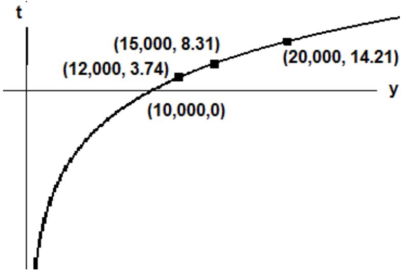
If we consider just the function \(t = g(y) = \dfrac{\ln\!\left(\dfrac{y}{10000}\right)}{\ln(1.05)}\) mathematically, then the domain of the function would be \(y > 0\) (all positive real numbers), and the range for \(t\) would be all real numbers.
However, in the context of this investment problem, the initial investment at time \(t = 0\) is \(y = \$10{,}000\). Negative values for time do not make sense. Values of the investment that are lower than the initial amount of \(\$10{,}000\) also do not make sense for an investment that is increasing in value.
This is a great example of how mathematical functions need to be interpreted in context. Mathematically, we could plug in \(y = 5000\) and get a negative time value, but that would mean "the investment was worth $5,000 at some point in the past." Since we're modeling future growth from a starting point of $10,000, we restrict our domain and range to values that make practical sense.
Therefore, the function and graph as it pertains to this problem concerning investments has domain \(y \geq 10000\) and range \(t \geq 0\).
The graph below is restricted to the domain and range that make practical sense for the investment in this problem:
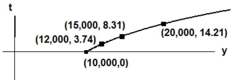
Look at how the curve flattens out as the investment value increases. This tells us that each additional dollar of growth takes progressively longer to achieve. To double your money from $10,000 to $20,000 takes about 14 years, but to go from $20,000 to $30,000 (the same $10,000 increase) takes even longer. This is why financial advisors emphasize starting to save early—time is your most valuable asset in investing.
Converting Between Exponential Forms
Why do we need to convert between these two forms? In real-world applications, different forms of exponential functions are useful in different contexts. The form \(y = ae^{kt}\) is common in continuous growth models (like population growth or radioactive decay), while the form \(y = ab^t\) is often easier to interpret when dealing with discrete time periods (like annual interest rates). Being able to convert between them lets you choose the most useful representation for your specific problem.
Converting between exponential forms:
- If the function is given in the form \(y = ae^{kt}\), rewrite it in the form \(y = ab^t\).
- If the function is given in the form \(y = ab^t\), rewrite it in the form \(y = ae^{kt}\).
The key relationship connecting these forms is \(b = e^k\). This means if you know \(k\), you can find \(b\) by calculating \(e^k\). Conversely, if you know \(b\), you can find \(k\) by calculating \(\ln(b)\). This connection comes from the fundamental property that \(e^{kt} = (e^k)^t\).
Section 5.5 Problem Set: Applications of Exponential and Logarithmic Functions
These problems bring together everything you've learned about exponential growth, exponential decay, and logarithms. You'll work with real-world scenarios like investments, population changes, medication dosages, and depreciation. The key skill here is recognizing which type of exponential model fits each situation, then using logarithms to solve for unknown time values. Think of these as your toolkit for predicting the future based on percentage rates of change.
When you see phrases like "increasing at a rate of X% per year" or "decreasing at a rate of Y% per year," you're dealing with exponential models. The growth factor is \((1 + r)\) for growth and \((1 - r)\) for decay, where \(r\) is the rate as a decimal. If you need to find "when" something happens, you'll use logarithms to solve for time.
1) An investment's value is rising at the rate of 5% per year. The initial value of the investment is $20,000 in 2016.
- Write the function that gives the value of the investment as a function of time \(t\) in years after 2016.
- Find the value of the investment in 2028.
- When will the value be $30,000?
Problem 1 Solution
Part a: Write the exponential growth function.
Step 1: Identify the given information.
- Initial value: \(a = 20000\)
- Growth rate: \(r = 0.05\) (5% as a decimal)
- Growth factor: \(b = 1 + r = 1 + 0.05 = 1.05\)
Step 2: Write the exponential growth function using \(y = ab^t\).
\[y = 20000(1.05)^t\]where \(t\) is the number of years after 2016.
Answer (Part a): \(y = 20000(1.05)^t\)
Part b: Find the value in 2028.
Step 1: Determine the time elapsed. From 2016 to 2028 is \(t = 2028 - 2016 = 12\) years.
Step 2: Substitute \(t = 12\) into the function and evaluate.
\[y = 20000(1.05)^{12}\] \[y = 20000(1.7959)\] \[y = 35918\]Answer (Part b): The investment will be worth $35,918 in 2028.
Verification: Starting with $20,000 and growing at 5% per year for 12 years: \(20000 \times 1.05^{12} = 35918\) ✓
Part c: When will the value be $30,000?
Step 1: Set up the equation with \(y = 30000\) and solve for \(t\).
\[30000 = 20000(1.05)^t\]Step 2: Divide both sides by 20000 to isolate the exponential expression.
\[\frac{30000}{20000} = (1.05)^t\] \[1.5 = (1.05)^t\]Step 3: The variable is in the exponent, so use logarithms. Rewrite in logarithmic form.
\[t = \log_{1.05}(1.5)\]Step 4: Use the change of base formula with natural logarithms.
\[t = \frac{\ln(1.5)}{\ln(1.05)} = \frac{0.4055}{0.0488} = 8.31 \text{ years}\]Answer (Part c): The investment will reach $30,000 after approximately 8.31 years (around mid-2024).
Verification: \(20000(1.05)^{8.31} = 20000(1.5001) = 30002 \approx 30000\) ✓
2) The population of a city is increasing at the rate of 2.3% per year, since the year 2000. Its population in 2010 was 137,000 people. Find the population of the city in the year 2000.
Problem 2 Solution
Step 1: Identify the given information and what we're solving for.
- Growth rate: \(r = 0.023\) (2.3% as a decimal)
- Growth factor: \(b = 1 + r = 1 + 0.023 = 1.023\)
- Population in 2010: \(y = 137000\) when \(t = 10\) years after 2000
- Unknown: initial population \(a\) in the year 2000
Step 2: Write the exponential growth model.
\[y = a(1.023)^t\]Step 3: Substitute the known values (\(y = 137000\) when \(t = 10\)).
\[137000 = a(1.023)^{10}\]Step 4: This is Strategy B—the variable is the coefficient. First evaluate \((1.023)^{10}\).
\[(1.023)^{10} = 1.2553\]Step 5: Solve the resulting linear equation for \(a\).
\[137000 = a(1.2553)\] \[a = \frac{137000}{1.2553} = 109{,}134\]Answer: The population of the city in the year 2000 was approximately 109,134 people.
Verification: Starting with 109,134 and growing at 2.3% per year for 10 years: \(109134 \times 1.023^{10} = 109134 \times 1.2553 = 137{,}000\) ✓
3) The value of a piece of industrial equipment depreciates after it is purchased. Suppose that the depreciation follows an exponential decay model. The value of the equipment at the end of 8 years is $30,000 and its value has been decreasing at the rate of 7.5% per year.
Find the initial value of the equipment when it was purchased.
Problem 3 Solution
Step 1: Identify the given information.
- Decay rate: \(r = -0.075\) (7.5% decrease as a decimal)
- Decay factor: \(b = 1 + r = 1 + (-0.075) = 0.925\)
- Value after 8 years: \(y = 30000\) when \(t = 8\)
- Unknown: initial value \(a\)
Step 2: Write the exponential decay model.
\[y = a(0.925)^t\]Step 3: Substitute the known values (\(y = 30000\) when \(t = 8\)).
\[30000 = a(0.925)^8\]Step 4: This is Strategy B—the variable is the coefficient. First evaluate \((0.925)^8\).
\[(0.925)^8 = 0.5490\]Step 5: Solve the resulting linear equation for \(a\).
\[30000 = a(0.5490)\] \[a = \frac{30000}{0.5490} = 54{,}645\]Answer: The initial value of the equipment when purchased was approximately $54,645.
Verification: Starting with $54,645 and depreciating at 7.5% per year for 8 years: \(54645 \times 0.925^8 = 54645 \times 0.5490 = 30{,}000\) ✓
4) An investment has been losing money. Its value has been decreasing at the rate of 3.2% per year. The initial value of the investment was $75,000 in 2010.
- Write the function that gives the value of the investment as a function of time \(t\) in years after 2010.
- If the investment's value continues to decrease at this rate, find the value of the investment in 2020.
Problem 4 Solution
Part a: Write the exponential decay function.
Step 1: Identify the given information.
- Initial value: \(a = 75000\)
- Decay rate: \(r = -0.032\) (3.2% decrease as a decimal)
- Decay factor: \(b = 1 + r = 1 + (-0.032) = 0.968\)
Step 2: Write the exponential decay function using \(y = ab^t\).
\[y = 75000(0.968)^t\]where \(t\) is the number of years after 2010.
Answer (Part a): \(y = 75000(0.968)^t\)
Part b: Find the value in 2020.
Step 1: Determine the time elapsed. From 2010 to 2020 is \(t = 10\) years.
Step 2: Substitute \(t = 10\) into the function and evaluate.
\[y = 75000(0.968)^{10} = 75000(0.7224) = 54{,}180\]Answer (Part b): The investment will be worth approximately $54,180 in 2020.
Verification: \(75000 \times 0.968^{10} = 75000 \times 0.7224 = 54{,}180\) ✓
5) A social media site has 275 members initially. The number of members has been increasing exponentially according to the function \(y = 275e^{0.21t}\), where \(t\) is the number of months since the site's initial launch. How many months does it take until the site has 5000 members? State answer to the nearest tenth of a month (1 decimal place).
Problem 5 Solution
Step 1: Identify the given information.
- Exponential growth function: \(y = 275e^{0.21t}\)
- Target membership: \(y = 5000\)
- Unknown: time \(t\) in months
Step 2: Substitute \(y = 5000\) into the equation.
\[5000 = 275e^{0.21t}\]Step 3: Divide both sides by 275 to isolate the exponential expression.
\[\frac{5000}{275} = e^{0.21t}\] \[18.182 = e^{0.21t}\]Step 4: The variable is in the exponent with base \(e\), so use natural logarithms.
\[0.21t = \ln(18.182)\]Step 5: Solve for \(t\).
\[t = \frac{\ln(18.182)}{0.21} = \frac{2.9004}{0.21} = 13.8 \text{ months}\]Answer: It takes approximately 13.8 months for the site to reach 5000 members.
Verification: \(275e^{0.21(13.8)} = 275e^{2.898} = 275(18.15) = 4991 \approx 5000\) ✓
6) A city has a population of 62,000 people in the year 2000. Due to high unemployment, the city's population has been decreasing at the rate of 2% per year. Using this model, find the population of this city in 2016.
Problem 6 Solution
Step 1: Identify the given information.
- Initial population (year 2000): \(a = 62000\)
- Decay rate: \(r = -0.02\) (2% decrease as a decimal)
- Decay factor: \(b = 1 + r = 1 + (-0.02) = 0.98\)
- Time elapsed: From 2000 to 2016 is \(t = 16\) years
Step 2: Write the exponential decay model.
\[y = 62000(0.98)^t\]Step 3: Substitute \(t = 16\) and evaluate.
\[y = 62000(0.98)^{16} = 62000(0.7238) = 44{,}876\]Answer: The population of the city in 2016 is approximately 44,876 people.
Verification: \(62000 \times 0.98^{16} = 62000 \times 0.7238 = 44{,}876\) ✓
7) A city has a population of 87,000 people in the year 2000. The city's population has been increasing at the rate of 1.5% per year. How many years does it take until the population reaches 100,000 people?
Problem 7 Solution
Step 1: Identify the given information.
- Initial population: \(a = 87000\)
- Growth rate: \(r = 0.015\) (1.5% as a decimal)
- Growth factor: \(b = 1 + r = 1 + 0.015 = 1.015\)
- Target population: \(y = 100000\)
- Unknown: time \(t\) in years
Step 2: Write the exponential growth model and substitute \(y = 100000\).
\[100000 = 87000(1.015)^t\]Step 3: Divide both sides by 87000.
\[\frac{100000}{87000} = (1.015)^t\] \[1.1494 = (1.015)^t\]Step 4: The variable is in the exponent, so use logarithms.
\[t = \log_{1.015}(1.1494) = \frac{\ln(1.1494)}{\ln(1.015)} = \frac{0.1393}{0.0149} = 9.35 \text{ years}\]Answer: It takes approximately 9.35 years for the population to reach 100,000 people (around the year 2009).
Verification: \(87000(1.015)^{9.35} = 87000(1.1495) = 100{,}007 \approx 100{,}000\) ✓
8) An investment of $50,000 is increasing in value at the rate of 6.3% per year. How many years does it take until the investment is worth $70,000?
Problem 8 Solution
Step 1: Identify the given information.
- Initial value: \(a = 50000\)
- Growth rate: \(r = 0.063\) (6.3% as a decimal)
- Growth factor: \(b = 1 + r = 1 + 0.063 = 1.063\)
- Target value: \(y = 70000\)
- Unknown: time \(t\) in years
Step 2: Set up and solve the exponential equation.
\[70000 = 50000(1.063)^t\] \[\frac{70000}{50000} = (1.063)^t\] \[1.4 = (1.063)^t\]Step 3: Use logarithms (change of base formula).
\[t = \frac{\ln(1.4)}{\ln(1.063)} = \frac{0.3365}{0.0611} = 5.51 \text{ years}\]Answer: It takes approximately 5.51 years for the investment to reach $70,000.
Verification: \(50000(1.063)^{5.51} = 50000(1.4002) = 70{,}010 \approx 70{,}000\) ✓
Problems 9–12 are "reverse engineering" problems. Instead of being given the rate and asked to find a future value, you're given two data points and asked to find the rate. This is where logarithms become essential. You'll set up an exponential equation with the unknown rate, then use logarithms to isolate and solve for that rate. These problems mirror real-world data analysis where you observe changes over time and need to determine the underlying growth or decay rate.
9) A city has a population of 50,000 people in the year 2000. The city's population increases at a constant percentage rate. Fifteen years later, in 2015, the population of this city was 70,000. Find the annual percentage growth rate.
Problem 9 Solution
Step 1: Identify the given information.
- Initial population: \(a = 50000\)
- Population after 15 years: \(y = 70000\) when \(t = 15\)
- Unknown: growth rate \(r\) (and growth factor \(b = 1 + r\))
Step 2: Write and substitute into the exponential growth model.
\[70000 = 50000(1 + r)^{15}\]Step 3: Divide both sides by 50000.
\[\frac{70000}{50000} = (1 + r)^{15}\] \[1.4 = (1 + r)^{15}\]Step 4: The variable is in the base, so take the 15th root of both sides.
\[\sqrt[15]{1.4} = 1 + r\] \[1.4^{1/15} = 1 + r\] \[1.0229 = 1 + r\]Step 5: Solve for \(r\).
\[r = 1.0229 - 1 = 0.0229\]Answer: The annual percentage growth rate is approximately 2.29% per year.
Verification: \(50000(1.0229)^{15} = 50000(1.4001) = 70{,}005 \approx 70{,}000\) ✓
10) 200 mg of a medication is administered to a patient. After 3 hours, only 100 mg remains in the bloodstream. Using an exponential decay model, find the hourly decay rate.
Problem 10 Solution
Step 1: Identify the given information.
- Initial amount: \(a = 200\) mg
- Amount after 3 hours: \(y = 100\) mg when \(t = 3\)
- Unknown: decay rate \(r\) (and decay factor \(b = 1 + r\))
Step 2: Write and substitute into the exponential decay model.
\[100 = 200(1 + r)^3\]Step 3: Divide both sides by 200.
\[\frac{100}{200} = (1 + r)^3\] \[0.5 = (1 + r)^3\]Step 4: The variable is in the base, so take the cube root of both sides.
\[\sqrt[3]{0.5} = 1 + r\] \[0.5^{1/3} = 1 + r\] \[0.7937 = 1 + r\]Step 5: Solve for \(r\).
\[r = 0.7937 - 1 = -0.2063\]Answer: The hourly decay rate is approximately 20.63% per hour (or \(r = -0.2063\) as a decimal).
Verification: \(200(0.7937)^3 = 200(0.5000) = 100\) mg ✓
11) An investment is losing money at a constant percentage rate per year. The investment was initially worth $25,000 but is worth only $20,000 after 4 years. Find the percentage rate at which the investment is losing value each year (that is, find the annual decay rate).
Problem 11 Solution
Step 1: Identify the given information.
- Initial value: \(a = 25000\)
- Value after 4 years: \(y = 20000\) when \(t = 4\)
- Unknown: decay rate \(r\) (and decay factor \(b = 1 + r\))
Step 2: Write and substitute into the exponential decay model.
\[20000 = 25000(1 + r)^4\]Step 3: Divide both sides by 25000.
\[\frac{20000}{25000} = (1 + r)^4\] \[0.8 = (1 + r)^4\]Step 4: The variable is in the base, so take the 4th root of both sides.
\[\sqrt[4]{0.8} = 1 + r\] \[0.8^{1/4} = 1 + r\] \[0.9457 = 1 + r\]Step 5: Solve for \(r\).
\[r = 0.9457 - 1 = -0.0543\]Answer: The annual decay rate is approximately 5.43% per year (or \(r = -0.0543\) as a decimal).
Verification: \(25000(0.9457)^4 = 25000(0.8000) = 20{,}000\) ✓
12) Using the information in question 11, how many years does it take until the investment is worth only half of its initial value?
Problem 12 Solution
Step 1: Use the information from Problem 11.
- Initial value: \(a = 25000\)
- Decay factor: \(b = 0.9457\) (from Problem 11)
- Target value: \(y = \frac{1}{2}(25000) = 12500\) (half the initial value)
- Unknown: time \(t\) in years
Step 2: Write the exponential decay model using the decay factor from Problem 11.
\[12500 = 25000(0.9457)^t\]Step 3: Divide both sides by 25000.
\[\frac{12500}{25000} = (0.9457)^t\] \[0.5 = (0.9457)^t\]Step 4: Use logarithms (change of base formula).
\[t = \frac{\ln(0.5)}{\ln(0.9457)} = \frac{-0.6931}{-0.0558} = 12.42 \text{ years}\]Answer: It takes approximately 12.42 years for the investment to be worth half of its initial value.
Verification: \(25000(0.9457)^{12.42} = 25000(0.5000) = 12{,}500\) ✓
After working through these problems, you'll have practiced the full cycle of exponential modeling: writing functions from word problems, evaluating them at specific times, solving for time using logarithms, and finding unknown rates from data. These skills apply directly to finance, biology, chemistry, economics, and any field where things change at a constant percentage rate over time.
13a) \(y = 7900e^{0.472t}\). Write in the form \(y = ab^t\).
Problem 13a Solution
Step 1: Identify the relationship between the two forms.
We know that \(y = ae^{kt} = ab^t\), which means \(a(e^k)^t = ab^t\), therefore: \(b = e^k\)
Step 2: In this problem, \(k = 0.472\), so calculate \(b\).
\[b = e^{0.472} = 1.603\]Step 3: Write the function in the form \(y = ab^t\).
\[y = 7900(1.603)^t\]Answer: \(y = 7900(1.603)^t\)
Verification: For \(t = 1\): \(7900e^{0.472(1)} = 7900(1.603) = 12{,}664\) ✓
13b) \(y = 4567(0.67)^t\). Write in the form \(y = ae^{kt}\).
Problem 13b Solution
Step 1: Identify the relationship between the two forms.
We know that \(y = ae^{kt} = ab^t\), which means \(e^k = b\), so \(k = \ln(b)\).
Step 2: In this problem, \(b = 0.67\), so calculate \(k\).
\[k = \ln(0.67) = -0.4005\]Step 3: Write the function in the form \(y = ae^{kt}\).
\[y = 4567e^{-0.4005t}\]Answer: \(y = 4567e^{-0.4005t}\)
Verification: For \(t = 1\): \(4567(0.67)^1 = 4567e^{-0.4005(1)} = 4567(0.67) = 3{,}060\) ✓
13c) \(y = 18720(1.47)^t\). Write in the form \(y = ae^{kt}\).
Problem 13c Solution
Step 1: Identify the relationship between the two forms.
We know that \(e^k = b\), so \(k = \ln(b)\).
Step 2: In this problem, \(b = 1.47\), so calculate \(k\).
\[k = \ln(1.47) = 0.3853\]Step 3: Write the function in the form \(y = ae^{kt}\).
\[y = 18720e^{0.3853t}\]Answer: \(y = 18720e^{0.3853t}\)
Verification: For \(t = 1\): \(18720(1.47)^1 = 18720e^{0.3853(1)} = 18720(1.47) = 27{,}518\) ✓
13d) \(y = 1200e^{-0.078t}\). Write in the form \(y = ab^t\).
Problem 13d Solution
Step 1: Identify the relationship between the two forms.
We know that \(b = e^k\).
Step 2: In this problem, \(k = -0.078\), so calculate \(b\).
\[b = e^{-0.078} = 0.9249\]Step 3: Write the function in the form \(y = ab^t\).
\[y = 1200(0.9249)^t\]Answer: \(y = 1200(0.9249)^t\)
Verification: For \(t = 1\): \(1200e^{-0.078(1)} = 1200(0.9249) = 1{,}110\) ✓
Section 5.6 Problem Set: Chapter Review
This chapter review brings together all the exponential growth and decay concepts you've learned. These problems mirror real-world scenarios you'll encounter in finance, biology, medicine, and demographics. Take your time with each problem—they're designed to test your understanding of when to use exponential models and how to manipulate them to find what you need.
1) The value of a new boat depreciates after it is purchased. The value of the boat 7 years after it was purchased is $25,000 and its value has been decreasing at the rate of 8.2% per year.
- Find the initial value of the boat when it was purchased.
- How many years after it was purchased will the boat's value be $20,000?
- What was its value 3 years after the boat was purchased?
Depreciation problems work backward from a known value at a specific time. You're essentially "rewinding" the exponential decay to find the starting point. This is common in accounting and tax calculations for vehicles and equipment.
2) Tony invested $40,000 in 2010; unfortunately his investment has been losing value at the rate of \(2.7\%\) per year.
- Write the function that gives the value of the investment as a function of time \(t\) in years after 2010.
- Find the value of the investment in 2020, if its value continues to decrease at this rate.
- In what year will the investment be worth half its original value?
The "half-life" question in part (c) is a classic exponential decay problem. Whether it's radioactive material, medication in your bloodstream, or a declining investment, the mathematics is identical. The half-life formula gives you a quick way to understand how fast something is disappearing.
3) Rosa invested $25,000 in 2005; its value has been increasing at the rate of 6.4% annually.
- Write the function that gives the value of the investment as a function of time \(t\) in years after 2005.
- Find the value of the investment in 2025.
A 6.4% annual return is quite good for a long-term investment! This problem shows the power of compound growth over 20 years. Even though the percentage seems modest, the cumulative effect is substantial—this is why financial advisors emphasize starting to invest early.
4) The population of a city is increasing at the rate of \(3.2\%\) per year, since the year 2000. Its population in 2015 was 235,000 people.
- Find the population of the city in the year 2000.
- In what year will the population be 250,000 if it continues to grow at this rate?
- What was the population of this city in the year 2008?
Urban planners use these exact calculations to predict infrastructure needs. If you know a city is growing at 3.2% annually, you can forecast when you'll need more schools, hospitals, roads, and water treatment facilities. The exponential model helps governments plan decades in advance.
5) The population of an endangered species has only 5,000 animals now. Its population has been decreasing at the rate of \(12\%\) per year.
- If the population continues to decrease at this rate, how many animals will be in this population 4 years from now?
- In what year will there be only 2,000 animals remaining in this population?
A 12% annual decline is alarming for conservationists. This problem illustrates why wildlife biologists track population trends so carefully—exponential decay can drive a species to critically low numbers surprisingly fast. Understanding the math helps conservation organizations prioritize which species need immediate intervention.
6) \(300\text{ mg}\) of a medication is administered to a patient. After 5 hours, only \(80\text{ mg}\) remains in the bloodstream.
- Using an exponential decay model, find the hourly decay rate.
- How many hours after the \(300\text{ mg}\) dose of medication was administered was there \(125\text{ mg}\) in the bloodstream?
- How much medication remains in the bloodstream after 8 hours?
Pharmacokinetics—the study of how drugs move through the body—relies heavily on exponential decay models. Doctors use these calculations to determine dosing schedules. If a medication decays too quickly, you need multiple doses per day. If it decays slowly, you might only need one dose daily. Getting this wrong can mean the drug is either ineffective or toxic.
7) If \(y = 240b^t\) and \(y = 600\) when \(t = 6\) years, find the annual growth rate. State your answer as a percent.
This problem gives you the exponential function structure but asks you to work backward to find the base \(b\), which represents the growth factor. Once you have \(b\), converting it to a percentage growth rate is straightforward: if \(b = 1.08\), the growth rate is 8%. This skill is essential for analyzing any exponential data where you know the starting point and a later value.
8) If the function is given in the form \(y = ae^{kt}\), rewrite it in the form \(y = ab^{t}\). If the function is given in the form \(y = ab^{t}\), rewrite it in the form \(y = ae^{kt}\).
- \(y = 375000(1.125^{t})\)
- \(y = 5400e^{0.127t}\)
- \(y = 230e^{-0.62t}\)
- \(y = 3600(0.42^{t})\)
These two forms—\(y = ab^t\) and \(y = ae^{kt}\)—are mathematically equivalent, just different ways of expressing the same exponential relationship. The base-\(e\) form (\(y = ae^{kt}\)) is preferred in calculus and continuous growth models because it makes derivatives cleaner. The base-\(b\) form (\(y = ab^t\)) is more intuitive for discrete time periods like annual growth. Being fluent in both forms lets you choose the most convenient one for your problem.
The conversion formulas are:
- From \(y = ab^t\) to \(y = ae^{kt}\): Use \(k = \ln(b)\)
- From \(y = ae^{kt}\) to \(y = ab^t\): Use \(b = e^k\)
Looking Ahead: Chapter Preview
In the next chapter, you will learn to:
- Solve financial problems that involve simple interest.
- Solve problems involving compound interest.
- Find the future value of an annuity, and the amount of payments to a sinking fund.
- Find the present value of an annuity, and an installment payment on a loan.
You've just mastered exponential functions—the mathematical foundation for understanding how money grows over time. The next chapter applies these concepts directly to personal finance: savings accounts, loans, mortgages, and retirement planning. Everything you've learned about exponential growth and decay will now help you make smarter financial decisions in your own life.